Example of Cascaded Integrator Comb filter in Matlab

Equivalence of Moving Average and CIC filter

Let me briefly share my understanding on the cascaded integrator comb (CIC) filter, thanks to the nice article. For understanding the cascaded integrator comb (CIC) filter, firstly let us understand the moving average filter, which is accumulation latest samples of an input sequence .

Figure: Moving average filter

The frequency response of the moving average filter is:

.

% Moving Average filter
N = 10;
xn = sin(2*pi*[0:.1:10]);
hn = ones(1,N);
y1n = conv(xn,hn);

% transfer function of Moving Average filter
hF = fft(hn,1024);
plot([-512:511]/1024, abs(fftshift(hF)));
xlabel(‘Normalized frequency’)
ylabel(‘Amplitude’)
title(‘frequency response of Moving average filter’)

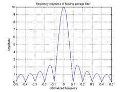
Figure: Frequency response of moving average filter

The moving average filter which is implemented as a direct form FIR type as shown above can also be implemented in a recursive form. It consists of a comb stage whose output is difference of the current sample and the sample which cameprior. The difference is successively accumulated by an integrator stage. Together the circuits behave identically as the moving average filter described prior.

It can be proved using a simple proof that:

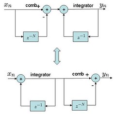
Figure: Cascaded Integrator Comb Filter

Bit more details can be found in Sec2.5.2 Recursive and Non Recursive Realization of FIR systems in [DSP-PROAKIS].

As the system is linear, the position of the integrator and comb stage can be swapped. Now, using a small Matlab code snippet let us verify that the output from CIC realization is indeed the same as obtained from moving average filter.

% Implementing Cascaded Integrator Comb filter with the
% comb section following the integrator stage
N = 10;
delayBuffer = zeros(1,N);
intOut = 0;
xn = sin(2*pi*[0:.1:10]);
for ii = 1:length(xn)
% comb section
combOut = xn(ii) – delayBuffer(end);
delayBuffer(2:end) = delayBuffer(1:end-1);
delayBuffer(1) = xn(ii);

% integrator
intOut = intOut + combOut;
y2n(ii) = intOut;
end

err12 = y1n(1:length(xn)) – y2n;
err12dB = 10*log10(err12*err12′/length(err12)) % identical outputs
close all

% Implementing Cascaded Integrator Comb filter with the
% integrator section following the comb stage

N = 10;
delayBuffer = zeros(1,N);
intOut = 0;
xn = sin(2*pi*[0:.1:10]);
for ii = 1:length(xn)
% integrator
intOut = intOut + xn(ii);

% comb section
combOut = intOut – delayBuffer(end);
delayBuffer(2:end) = delayBuffer(1:end-1);
delayBuffer(1) = intOut;
y3n(ii) = combOut;

end
err13 = y1n(1:length(xn)) – y3n;
err13dB = 10*log10(err13*err13′/length(err13)) % identical outputs

The outputs are matching.

The recursive realization of the FIR filter as described above helps to achieve the same result with less hardware.

Using CIC filter for decimation

Typically, decimation to a lower sampling rate is achieved by taking one sample out of every samples. There exists an anti-aliasing filter to remove the un-desired spectrum before decimation.

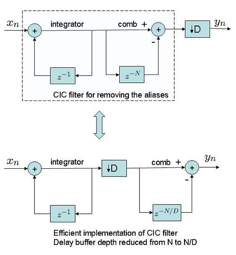
Figure: CIC filters for decimation

As shown above, the same output can be achieved by having the decimation stage between integrator stage and comb stage. This helps in reducing the delay buffer depth requirement of the comb section. Using a small Matlab code snippet, let us check whether both the implementations behave identically.

% For decimation, having the CIC filtering before taking every other sample
D = 2; % decimation factor
N = 10; % delay buffer depth
delayBuffer = zeros(1,N); % init
intOut = 0;
xn = sin(2*pi*[0:.1:10]);
y6n = [];
for ii = 1:length(xn)
% comb section
combOut = xn(ii) – delayBuffer(end);
delayBuffer(2:end) = delayBuffer(1:end-1);
delayBuffer(1) = xn(ii);

% integrator
intOut = intOut + combOut;
y6n = [y6n intOut];

end
y6n = y6n(1:D:end); % taking every other sample – decimation

% For efficient hardware implementation of the CIC filter, having the
% integrator section first, decimate, then the comb stage
% Gain : Reduced the delay buffer depth of comb section from N to N/D
D = 2; % decimation factor
N = 10; % delay buffer depth
delayBuffer = zeros(1,N/D);
intOut = 0;
xn = sin(2*pi*[0:.1:10]); % input
y7n = []; % output
for ii = 1:length(xn)
% integrator
intOut = intOut + xn(ii);

if mod(ii,2)==1
% comb section
combOut = intOut – delayBuffer(end);
delayBuffer(2:end) = delayBuffer(1:end-1);
delayBuffer(1) = intOut;
y7n = [ y7n combOut];
end

end
err67 = y6n – y7n;
err67dB = 10*log10(err67*err67′/length(err67))

The outputs are matching.

Using CIC filters for interpolation

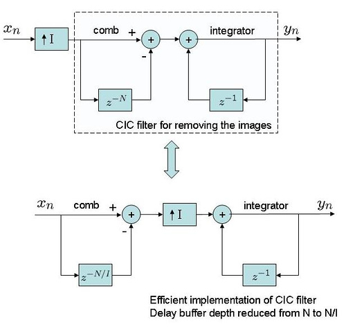
Typically, interpolation to a higher sampling rate achieved by inserting zeros between consecutive samples followed by filtering (for removing the images).

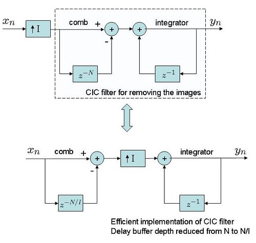
Figure: Using CIC filters for interpolation

As shown above, the same result can be achieved by having the upsampling stage between comb and integrator stage. This helps in reducing the delay buffer depth requirement of the comb section. Using a small Matlab code snippet, let us check whether both the implementations behave identically.

% For interpolation, insert the zeros followed by CIC filtering
xn = sin(2*pi*[0:.1:10]);
I = 2; % interpolation factor
N = 10; % filter buffer depth
xUn = [xn; zeros(1,length(xn))];
xUn = xUn(:).’; % zeros inserted
delayBuffer = zeros(1,N);
intOut = 0;
for ii = 1:length(xUn)
% comb section
combOut = xUn(ii) – delayBuffer(end);
delayBuffer(2:end) = delayBuffer(1:end-1);
delayBuffer(1) = xUn(ii);

% integrator
intOut = intOut + combOut;
y4n(ii) = intOut;

end

% For efficient hardware implementation of CIC filter for interpolation, having
% the comb section, then zeros insertion, followed by integrator section
% Gain : Reduced the delay buffer depth of comb section from N to N/I

I = 2; % interpolation factor
N = 10; % original delay buffer depth
delayBuffer = zeros(1,N/I); % new delay buffer of N/I
intOut = 0;
xn = sin(2*pi*[0:.1:10]);
y5n = [];
for ii = 1:length(xn)
% comb section
combOut = xn(ii) – delayBuffer(end);
delayBuffer(2:end) = delayBuffer(1:end-1);
delayBuffer(1) = xn(ii);

% upsampling
combOutU = [ combOut zeros(1,1)];

for jj =0:I-1
% integrator
intOut = intOut + combOutU(jj+1);
y5n = [y5n intOut];
end

end

err45 = y4n – y5n;
err45dB = 10*log10(err45*err45′/length(err45)) % outputs matching

The outputs are matching.

One one question: Upsampling by a factor which is achieved by repeating the sample times result in the same output as obtained by the CIC filter implementation described above (see previous post trying to describe that zero-order hold for interpolation). Considering so, do we need to have the filtering hardware when doing interpolation? I do not think so. If I have some additional thoughts, I will update.

References:

[1] Understanding cascaded integrator-comb filters – By Richard Lyons, Courtesy of Embedded Systems Programming URL: http://www.us.design-reuse.com/articles/article10028.html

[2] Digital Signal Processing – Principles, Algorithms and Applications, John G. Proakis, Dimitris G. Manolakis

Tagged as: CIC, decimation, interpolation

Related posts

1. Using Toeplitz matrices in MATLAB
2. Zero-order hold and first-order hold based interpolation
3. Polyphase filters for interpolation
4. Interpreting the output of fft() operation in Matlab
5. Update: Correction in Matlab code for raised cosine filter

D id you like this article? Make sure that you do not miss a new article by subscribing to RSS feed OR subscribing to e-mail newsletter. Note: Subscribing via e-mail entitles you to download the free e-Book on BER of BPSK/QPSK/16QAM/16PSK in AWGN.