Considering a typical scenario where there might exist a small phase offset between local oscillator between the transmitter and receiver.
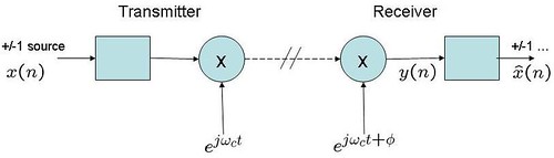
Figure 1 : Transmitter receiver with constant phase offset
In such cases, it might be desirable to estimate and track the phase offset such that the performance of the receiver does not degrade.
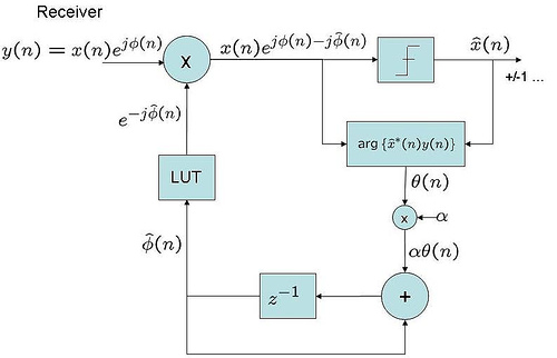
A simple first order digital phase locked loop for tracking the constat phase offset can be as
Assuming that the transmitter signal gets rotated by a constant phase
, the received signal
. In a simple no-noise case, assuming that the phase offset is small (and the signal gets decoded correctly), the estimate of phase offset is,
.
Typically, a first order phase locked loop which converges to is used for facilitating synchronous demodulation.
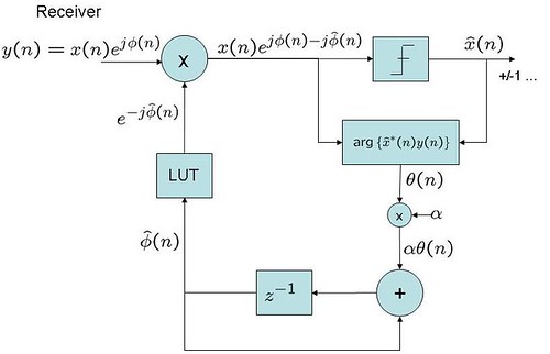
Figure 2 :
First order digital phase locked loop (PLL)
(adapted from Fig 5.7 of [Mengali])
The estimate from each sampling instant is accumulated to form the estimate
. This estimated phase is removed from the received samples
to generate
. The parameter
is a non-zero positive constant in the range
controls the rate of convergence of the loop. Higher value of
indicates faster convergence, but is more prone to noise effects. Lower value of
is less noisy, but results in slower convergence.
Assuming , the phase estimate at the output of the filter is
.
Substituting, , then
.
A simple Matlab code to simulate this can be as follows:
% random +/-1 BPSK source
xn = 2*(rand(1,1000) >0.5) - 1;
% introducing a phase offset of 20 degrees
phiDeg = 20;
phiRad = phiDeg*pi/180;
yn = xn*exp(j*phiRad);
% first order pll
alpha = 0.01;
phiHat = 0;
for ii = 1:length(yn)
   yn(ii) = yn(ii)*exp(-j*phiHat);
   % demodulating circuit
   xHat = 2*real(yn(ii)>0) -1 ;
   phiHatT = angle(conj(xHat)*yn(ii));
   % accumulation
   phiHat = alpha*phiHatT + phiHat;
   % dumping variables for plot
   phiHatDump(ii) = phiHat;
end

plot(phiHatDump*180/pi,'r.-')
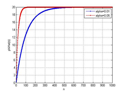
Figure 3: Convergence of for two
values.
Reference:
i tried this an worked. however, i would appreciate help in understanding what happened here…
% demodulating circuit
xHat = 2*real(x_n(ii)>0) – 1 ;
phiHatT = angle(conj(xHat)*x_n(ii)) – angle(conj(xHat)*xn(ii));
if phiHatT pi
phiHatT = -2*pi + phiHatT
end
% demodulating circuit
phiHatT = angle(x_n(ii)) – angle(xn(ii));
if phiHatT pi
phiHatT = -2*pi + phiHatT
end
works too…
i got it to work, but i still dont understand quite well what i said before. are you projecting an X axis or something like that? i really want to know. thank you.
look:
clc
clear all;
% sine wave
Tp = 1/60;
T = Tp/128;
Fp = 1/Tp;
Fs = 1/T;
w = 2*pi*Fp;
t = [0:T:809*T];
xn = sin(w*t);
%al simular con e^jwt siempre quedara una parte representada en coord imaginarias, por lo k habria k hacer unas modificaciones para que se detecte cuando no sea error de fase y sea causa de la misma onda.
%sin(wt+phi) = (e^jwt-e^-jwt)*e^phi/(2j)
% introducing a phase offset
phiDeg = -100;
phiRad = phiDeg*pi/180;
yn = xn*exp(j*phiRad);
% se puede representar un desfase cualquiera como e^j(wt+phi) ?
% first order pll
alpha = 0.05;
phiHat = 0;
x_n = zeros(length(t));
for ii = 1:length(t)
x_n(ii) = yn(ii)*exp(-j*phiHat);
% demodulating circuit
xHat = 2*real(x_n(ii)>0) – 1 ;
phiHatT = angle(conj(xHat)*x_n(ii)) – angle(conj(xHat)*xn(ii));
% accumulation
phiHat = alpha*phiHatT + phiHat;
% dumping variables for plot
phiHatDump(ii) = phiHat;
end
%plot(t,xn);
%hold on;
%plot(t,yn);
plot(t,phiHatDump*180/pi,’r.-‘);
it still wont work for angles above 90 degrees….
@Ananias: There are two assumptions
a) phase is constant
b) slicing of the received symbols is needed to remove the effect of modulation
Im trying to use this for a sine wave in the input. problem is it only works for 90 and -90. what can i do about it? i dont quite understand how you get the angle with
% demodulating circuit
xHat = 2*real(yn(ii)>0) -1 ;
phiHatT = angle(conj(xHat)*yn(ii));
@Ananias: Was the phase constant in the sinusoidal input?
Hi Krishna,
Can this code be used to recover the carrier ? Carrier signal is in 1GHz range.
Thank you
@Dinu: For recovering the carrier, we might need a second order loop. Will write about it soon.
Hi,
Thanks fr the reply Krishna. In the previous comment by Venkat, he describes quite similar scenario to my program. How can I check the accurancy of the code?
I have another question, I am working on low SNR environment. Does these phase lock loop work on low snr region?
Thanks in advance,
@Dinu: This piece of code does only phase tracking and not frequency tracking. I have not tried checking the performance in the low SNR region.
thanks
Hello Krishna,
I have referred your example on first order PLL for constant phase tracking.It was very useful.
https://dsplog.com/2007/06/10/first-order-digital-pll-for-tracking-constant-phase-offset/
But in the example a complex carrier is being used at the transmitter and receiver.Practically , when I use a cosine carrier at Tx. and cosine,sine carriers at Rx.(as in costas loop) , can the same loop filter be used ?
I have tried to simulate the above situation in the following script but was unable to estimate the phase. Please help me……….
% MODULATION
clc;
clear all;
close all;
[b,a] = butter(1,0.0156,’low’); % low pass filter to remove
nterm_i = 0; % double frequency component
dterm_i = 0;
nterm_q = 0;
dterm_q = 0;
n_sym = 10; % number of symbols
fs = 12.8e6;
t = 0:1/fs:100e-6 – 1/fs;
fc = fs/8; % carrier freuency
theta = 70*pi/180; % phase offset
r = 0.1e6; % symbol rate
oversamp = fs/r;
sym = randint(n_sym,1)*2-1;
in = 0;
for ind=1:1:n_sym
tmp(1:oversamp) = sym(ind);
in = [in tmp];
end
tx = in(2:end);
tx_carrier = cos(2*pi*fc*t + theta);
tx_out = tx.*tx_carrier;
% first order pll
alpha = 0.05;
phiHat = 0;
for ii = 1:1:length(t)
% Remove carrier
rx_i(ii) = tx_out(ii)*cos(2*pi*fc*t(ii) + phiHat);
rx_q(ii) = tx_out(ii)*sin(2*pi*fc*t(ii) + phiHat);
% low-pass IIR filter for I-channel
iir_in_i(ii) = rx_i(ii);
iir_out_i(ii) = b(1)*iir_in_i(ii)+ nterm_i + dterm_i;
nterm_i = b(2)*iir_in_i(ii);
dterm_i = a(2)*iir_out_i(ii);
% low-pass IIR filter for Q-channel
iir_in_q(ii) = rx_q(ii);
iir_out_q(ii) = b(1)*iir_in_q(ii)+ nterm_q + dterm_q;
nterm_q = b(2)*iir_in_q(ii);
dterm_q = a(2)*iir_out_q(ii);
% demodulating circuit
xHat = 2*(iir_out_i(ii)>0) -1 ; % symbol estimate
phiHatT =angle(conj(xHat)*rx_i(ii)); % phase error estimate angle(iir_out_i(ii) + i*iir_out_q(ii));%
% accumulation
phiHat = alpha*phiHatT + phiHat; % phase accumulator output
% dumping variables for plot
phiHatDump(ii) = phiHat;
end
plot(phiHatDump*180/pi,’-‘);
@venkat: Does your transmit signal contain phase information? Did the code work in no noise case?