 with transmit IQ gain/phase imbalance")
")
")
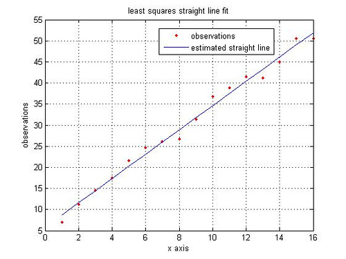
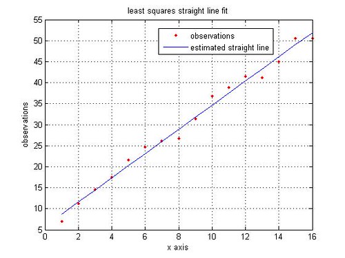
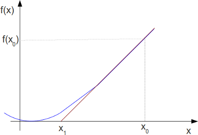
Two points suffice for drawing a straight line. However we may be presented with a set of data points (more than two?) presumably forming a straight line. How can one use the available set of data points to draw a straight line?
A probable approach is to draw a straight line which hopefully minimizes the error between the observed data points and estimated straight line.
where
is the observed data points and
is the points from estimated straight line.
To draw the estimated straight line , we need to estimate the slope,
and the constant,
.
Formulating as a matrix,
,
where,
=
is the set of observations is a matrix of dimension
,
=
is the set of coefficients is a matrix of dimension
,
is the slope and constant estimate of dimension
,
=
is the noise is a matrix of dimension
.
The least square estimate of the straight line is,
.
A simple MATLAB code for least squares straight line fit is given below:
% Least Squares Estimate
rand(‘state’,100); % initializing the random number generation
y = [5:3:50]; % observations, y_i
y = y + 5*rand(size(y)); % y_i with noise added
x = 1:length(y); % the x co-ordinates
% Formulating in matrix for solving for least squares estimate
Y = y.’;
X = [x.’ ones(1,length(x)).’];
alpha = inv(X’*X)*X’*Y; % solving for m and c
% constructing the straight line using the estimated slope and constant
yEst = alpha(1)*x + alpha(2);
close all
figure
plot(x,y,’r.’)
hold on
plot(x,yEst,’b’)
legend(‘observations’, ‘estimated straight line’)
grid on
ylabel(‘observations’)
xlabel(‘x axis’)
title(‘least squares straight line fit’)
References:
[1] Details on Curve fitting toolbox from MathWorks(TM) website
Fit a straight line trend & estimate the trend value for the year 2008 year : 2000, 2001, 2002, 2003, 2004, 2005, 2006 prod.: 110,112,115,119,121,123,1 26
@shashi: Hope you have solved this 🙂
@Sajith: Is this a homework assignment? In general, I prefer not to solve homework assignments, rather help you towards the solution. You can formulate the information in the least square matrix formultion explained in the post.
Year = [1971 1976 1977 1978 1979 1980 1981 1982]
Sales = [6.7 5.3 4.3 6.1 5.6 7.9 5.8 6.1]
X = [Year’ ones(8,1)]
Y = Sales.’
Once you have done that, then solution for slope and the constant is obtained by the leastsquares equation.
alpha = inv(X’*X)*X’*Y
Once you have the slope and constant, you can find the y-value (sales) for any x-value (year)
Hope this helps.
From the Data given below fit a straight line trend by the methord if least square and also estimate the sales for the year 1984.
Year 1971 1976 1977 1978 1979 1980 1981 1982
Sales 6.7 5.3 4.3 6.1 5.6 7.9 5.8 6.1
No special reason, except that when does this way, I have a reasonably clear idea of the underlying operations. Maybe helpful if I want to implement.
For the example above, the least squares solution can be obtained either by using X\Y or pinv(X)*Y. However, when X is rank-deficient, then the code in the post may fail and more ‘intelligent’ operations X\Y or pinv(X)*Y might be needed.
And a quick check showed that \ operator runs faster than pinv() or the code in the post.
Additionally, a nice thread in comp.dsp on this topic maybe interesting.
I find it interesting that you used inv and performed the matrix multiplication to solve this problem. Do you have a reason for doing it this way, instead of using MATLAB’s backslash operator (as in the linked material, below)?
Linear Regression in MATLAB
In curiosity,
Will